Depression Worldwide

Project "Dependence of Schizophrenia on different world development and healthcare systems indicators"

Authors:

Introduction

Mental health constitutes our emotions and feelings and it can affect our behavior, thoughts, and coping abilities [1]. The rate of mental health disorders is on a rise worldwide, due to modern society's chronic stress, demographic factors, substance abuse, and unhealthy lifestyles [2]. Nowadays, with less stigma, there is more recognition of the importance of mental health and how it can impact individuals in society. Schizophrenia is one type of mental health disorder that affects about 24 million individuals around the world. It is a chronic and severe mental illness that influences an individual's ability to think, feel, and behave clearly [3]. The symptoms of schizophrenia can be either positive or negative. Positive symptoms basically add, such as hallucinations, delusions, and distorted thinking or speech. Negative symptoms on the other hand can contribute to reduction. Negative symptoms can include, no emotion or motivation and social withdrawal [4]. The severity and type of symptoms can vary from person to person and can change over time.

Schizophrenia is a complex mental illness and its causes can be mainly due to chemical and neurotransmitter imbalances in the brain [5]. While there is no cure for Schizophrenia, researchers are trying to enhance their understanding of the underlying mechanisms and factors leading to the illness, and thus develop more effective and safer treatment options [4]. Several factors can trigger schizophrenia and impact its severity, including genetic predisposition, environmental factors, and substance use (i.e. cannabis). Stress and trauma can also exacerbate symptoms of schizophrenia and contribute to its severity [6].

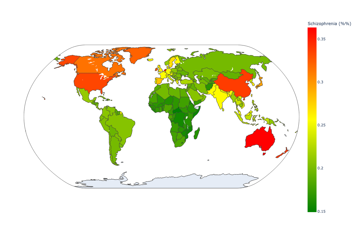Fig 1. Distribution of schozophrenia worldwide.

The distribution of schizophrenia is relatively uniform worldwide, with a prevalence of 1 in 300 (0.32%) in different regions [3]. However, significant disparities exist in access to mental health services and treatment for people with schizophrenia, especially in low- and middle-income and developing countries. Addressing these inequalities and ensuring that people with schizophrenia receive appropriate care and support is critical to improving outcomes and reducing the global burden of mental illness.

In this project, our main goal was to perform a multiple regression analysis to further enhance our understanding of the impact of different socioeconomic factors on the prevalence of schizophrenia around the world.

Dataset:

We collected our datasets in CSV format from the World Health Organization (WHO), which offers open-source data [7]. There were a total of 8 CSV files obtained from the WHO website:

MentalHealthDisorders.csv
WDIData_T.csv
Beds_in_mental_health_hospitals_per_100thousands.csv
Beds_for_mh_in_general_hospital_per100thousand_2019.csv
Psychologists_in_mental_health_per_100thousands.csv
Psychiatrists_in_mental_health.csv
Social_workers_in_mental_health_per_100thousands.csv
2.12_Health_systems.csv

To measure the impact of Schizophrenia within each society, the parameter of disability-adjusted life year (DALY) per 100,000 people is utilized. The DALY parameter is employed to gauge the total burden of depression. To compare countries using this parameter, the dataset "DALY” estimates WHO Member States by country. This dataset is sourced from the official World Health Organization website (http://who.int) and may be utilized for research purposes, with proper citation [7]. The dataset includes DALY parameters for each country in the WHO for every monitored disorder, segregated by gender and age, spanning the years from 2000 to 2019. For our project, we will utilize the data for Schizophrenia disorder from this dataset to find the indicators based on the DALY parameter.

The dataset about expenditures for the healthcare system worldwide is taken from The World Bank website [8]. This dataset contains health expenditures in percentage to Gross Domestic Product (GDP), expenditures in U.S. dollars, and expenditures in U.S. dollars per capita for 2019 by countries. This data is used in combination with the dataset "Government expenditures on mental health as a percentage of total government expenditures on health (%)" from the World Health Organization website [9]. By combining these data, we can analyze spending on mental health worldwide by country and the efficiency of spending on diagnostics and treatment in each healthcare system.

R code:

# Loading libraries
library(ggplot2)
library(olsrr)
library(dplyr)
library(lmtest)
library(mctest)
library(GGally)
library(MASS)
library(stats)

# Loading datasets
mhd <- read.csv('MentalHealthDisorders.csv')
wdi <- read.csv('WDIData_T.csv')
beds_mhh_p100t <- read.csv('beds_in_mental_health_hospitals_per_100thousands.csv')
beds_mhg_p100t <- read.csv('beds_for_mh_in_general_hospital_per100thousand_2019.csv')
psycho_p100t <- read.csv('psychologists_in_mental_health_per_100thousands.csv')
psychi_p100t <- read.csv('psychiatrists_in_mental_health.csv')
sw_p100t <- read.csv('social_workers_in_mental_health_per_100thousands.csv')

Methodology

We approached this project by running a linear regression model consisting of all the chosen independent variables to predict the most significant variables. For the purpose of this project, we selected data for only 2017.

R code:

mhd <- mhd[0:6468, ]
mhd2  <- mhd[mhd$Year == 2017  , ]
mhd2

The entire dataset with different World Development indicator contains more than 1400 indicators. For initial hypothesis about factors which can influence to the schizophrenia rate is the indicators should be from the following groups:

Economic factors, such as GDP, healthcare system expenditures
World development indicators. such as education indicators, urbanization, social factors, environmental indicators
Demographic indicators
HealthCare System indicators

At the first step it was decided to select these variables by 3 ways:

At first, some factors were selected to check by decision to understand is there any significant correlation between schizophrenia and such factors as:
GPD per capita
Current health expenditure per capita
Duration of education (primary and secondary)
Urban population (number and in % of total)
Secondly, for checking independent and significant variables the stepwise method was implemented for World Development Indicator dataset contained of more than 1400 indicators worldwide. By this method the next factors were selected:
Primary school starting age (years)
Rural population
Birth rate, crude (per 1,000 people)
People using at least basic drinking water services (% of population)
PM2.5 air pollution, population exposed to levels exceeding WHO guideline value (% of total)

Therefore, from dataset with World Development Indicators were selected next variables:

R code:

wdi2 = wdi[wdi$Year == 2017, ]
wdi_codes <- c('NY.GDP.PCAP.CD',
'SH.XPD.CHEX.PC.CD',
'SE.PRM.DURS',
'SE.SEC.DURS',
'SP.URB.TOTL.IN.ZS',
'SE.PRM.AGES',
'EN.ATM.PM25.MC.ZS',
'SP.RUR.TOTL',
'SH.H2O.BASW.ZS',
'SP.DYN.CBRT.IN',
'SP.URB.TOTL')
for (col in wdi_codes){
  print(paste(col, ':', wdi2[wdi2$IndicatorCode == col, ]$IndicatorName[3]))
}

Reshape World Development Indicators Data by creating separate column for each indicator.

R code:

Code1 = wdi_codes[1]
df_wdi = wdi2[wdi2$IndicatorCode == Code1, ][c('CountryCode', 'Year', 'Value')]
colnames(df_wdi) <- c( 'CountryCode', 'Year', Code1)
for (Code2 in wdi_codes[2:length(wdi_codes)])
{
  df2 = wdi2[wdi2$IndicatorCode == Code2, ][c('CountryCode', 'Year', 'Value')]
  colnames(df2) <- c('CountryCode', 'Year', Code2)
  df_wdi <- merge(x = df_wdi, y = df2, by = c('CountryCode', 'Year'), all = TRUE)
}

In addition, the healthcare systems indicators were selected from official WHO datasets (https://www.who.int/data/gho/data/indicators) :
Psychiatrists working in mental health sector (per 100,000)
Psychologists working in mental health sector (per 100,000)
Beds for mental health in general hospitals (per 100,000)
Beds in mental hospitals (per 100,000)

Merge these data with columns from WDI dataset and clean dataset from NA values

R code:

shizo <- mhd2[c('Year','Code', 'Schizophrenia....')]
colnames(shizo) <- c('Year','CountryCode', 'Schizo')
shizo$Schizo <- as.numeric(shizo$Schizo)
df3 <- merge(x = shizo, y = df_wdi, by = c('CountryCode', 'Year'))
df3 <- na.omit(df3[ , colSums(is.na(df3))<5])

df_temp <- psychi_p100t[c('SpatialDimValueCode', 'Value')]
colnames(df_temp) <- c('CountryCode', 'psychi_p100t')
df3 <- merge(x = df3, y = df_temp, by = c('CountryCode'), all = FALSE)
df_temp <- beds_mhh_p100t[c('SpatialDimValueCode', 'Value')]
colnames(df_temp) <- c('CountryCode', 'beds_mhh_p100t')
df3 <- merge(x = df3, y = df_temp, by = c('CountryCode'),  all = FALSE)
#df3 <- merge(x = df3, y = df_wdi, by = c('CountryCode', 'Year'), all = FALSE)
df_temp <- psycho_p100t[c('SpatialDimValueCode', 'Value')]
colnames(df_temp) <- c('CountryCode', 'psycho_p100t')
df3 <- merge(x = df3, y = df_temp, by = c('CountryCode'), all = FALSE)
df_temp <- beds_mhg_p100t[c('SpatialDimValueCode', 'Value')]
colnames(df_temp) <- c('CountryCode', 'beds_mhg_p100t')
df3 <- merge(x = df3, y = df_temp, by = c('CountryCode'),  all = FALSE)
df3 <- na.omit(df3)

For these parameters the linear model was created...:

R code:


dependent_variable <- 'Schizo'
independent_variables <- colnames(df3[5:length(df3)])
formula <- paste(dependent_variable, "~ (", paste(independent_variables, collapse=" + "), ')')
print(formula)
model <- lm(formula, data = df3)
summary(model)

... and the stepwise regression procedure was launched:

R code:

stepwise <-ols_step_both_p(model, pent = 0.1, prem = 0.3, details = FALSE)
print(stepwise$predictors)
dependent_variable <- 'Schizo'
independent_variables <- stepwise$predictors
for (col in independent_variables){
  print(paste(col, ':', wdi2[wdi2$IndicatorCode == col, ]$IndicatorName[3]))
}
formula2 <- paste(dependent_variable, "~(", paste(independent_variables, collapse=" + "), ')')

print(formula2)
model2 <- lm(formula2, data = df3)
summary(model2)

In the result only 6 variables were selected as independent and significant:

"EN.ATM.PM25.MC.ZS : PM2.5 air pollution, population exposed to levels exceeding WHO guideline value (% of total)"
"SH.H2O.BASW.ZS : People using at least basic drinking water services (% of population)"
"SE.PRM.AGES : Primary school starting age (years)"
"psycho_p100t : Psychologists working in mental health sector (per 100,000)"
"SP.URB.TOTL : Urban population"
"beds_mhh_p100t : Beds in mental hospitals (per 100,000)"

Interaction variables testing

model_h <- lm(Schizo ~ (EN.ATM.PM25.MC.ZS + SH.H2O.BASW.ZS + SE.PRM.AGES + psycho_p100t + SP.URB.TOTL + beds_mhh_p100t)^2, data = df3 )
summary(model_h)

The testing of model with interactions showed that no one of the interactions gives significant influence, but EN.ATM.PM25.MC.ZS:psycho_p100t gives the close to significant value and should be kept for next testing.

Higher order testing

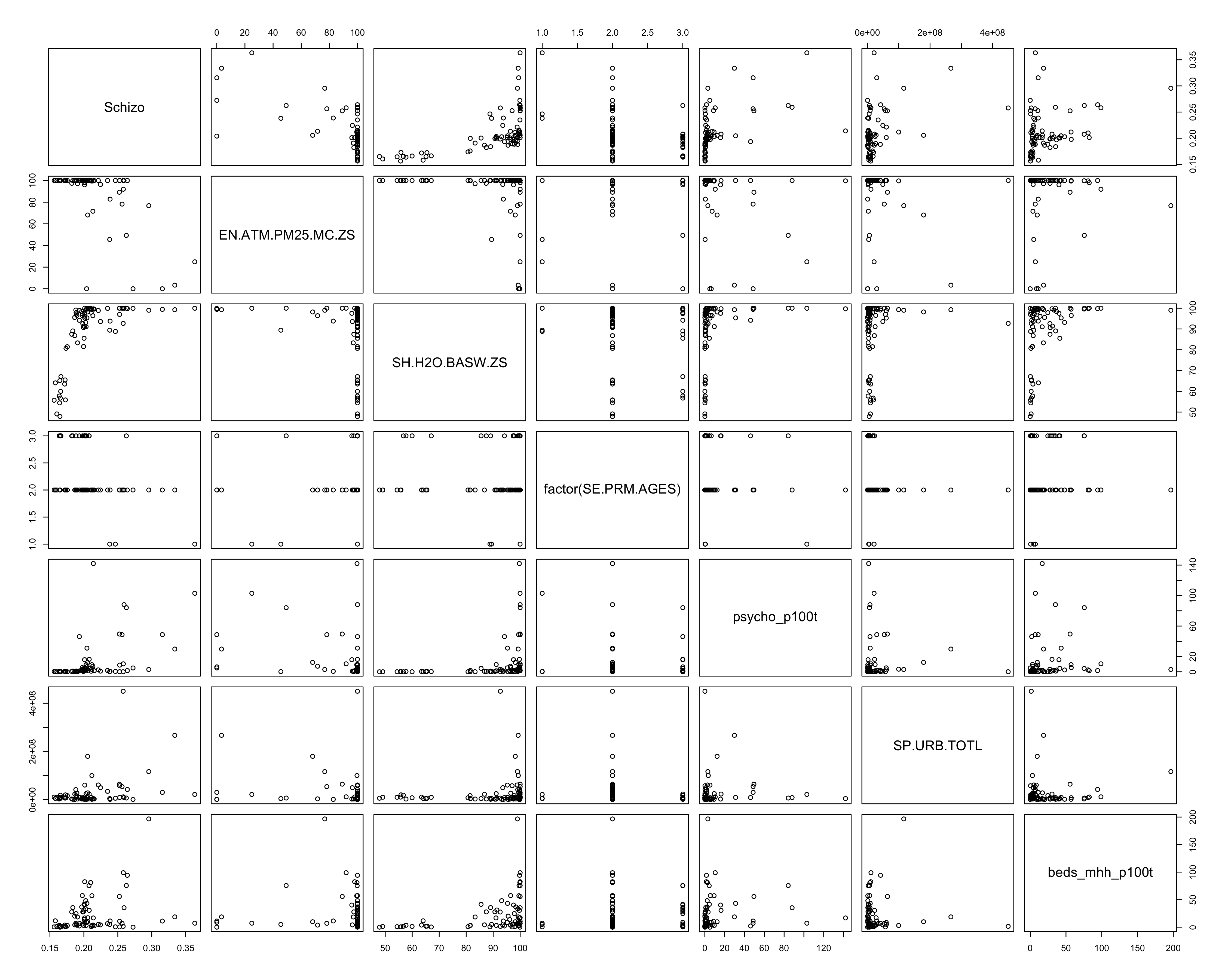Fig. 2. All pairwise combinations of variables

From the all pairwise combinations of variables there is only one variable which can be probable significant in higher order: psycho_p100k. Comparing the model with higher order of psycho_p100k and without we can hypothesize:
$H_0$ : Higher order term of psycho_p100k is not significant
$H_A$: Higher order of psycho_p100k is significant.

R code:

model_h <- lm(Schizo ~ EN.ATM.PM25.MC.ZS + SH.H2O.BASW.ZS + SE.PRM.AGES + psycho_p100t + I(psycho_p100t^2)+ SP.URB.TOTL + beds_mhh_p100t + EN.ATM.PM25.MC.ZS:psycho_p100t, data = df3 )
summary(model_h)

Result:

Call:
lm(formula = Schizo ~ EN.ATM.PM25.MC.ZS + SH.H2O.BASW.ZS + SE.PRM.AGES + 
    psycho_p100t + I(psycho_p100t^2) + SP.URB.TOTL + beds_mhh_p100t + 
    EN.ATM.PM25.MC.ZS:psycho_p100t, data = df3)

Residuals:
      Min        1Q    Median        3Q       Max 
-0.045033 -0.010802 -0.001732  0.009417  0.043419 

Coefficients:
                                 Estimate Std. Error t value Pr(>|t|)    
(Intercept)                     2.774e-01  3.455e-02   8.030 2.34e-11 ***
EN.ATM.PM25.MC.ZS              -3.751e-04  1.139e-04  -3.293 0.001598 ** 
SH.H2O.BASW.ZS                  8.437e-04  1.564e-04   5.395 9.98e-07 ***
SE.PRM.AGES                    -2.007e-02  4.449e-03  -4.511 2.72e-05 ***
psycho_p100t                    1.507e-03  3.095e-04   4.870 7.30e-06 ***
I(psycho_p100t^2)              -3.053e-06  2.302e-06  -1.326 0.189319    
SP.URB.TOTL                     1.343e-10  3.257e-11   4.123 0.000107 ***
beds_mhh_p100t                  2.492e-04  6.844e-05   3.642 0.000533 ***
EN.ATM.PM25.MC.ZS:psycho_p100t -9.971e-06  2.817e-06  -3.540 0.000740 ***
---
Signif. codes:  0 ‘***’ 0.001 ‘**’ 0.01 ‘*’ 0.05 ‘.’ 0.1 ‘ ’ 1

Residual standard error: 0.01733 on 66 degrees of freedom
Multiple R-squared:  0.8368,    Adjusted R-squared:  0.8171 
F-statistic: 42.31 on 8 and 66 DF,  p-value: < 2.2e-16

The testing of higher orders for different variables showed that the higher order variables gives not sifnificant influence. Therefore, it was decided not to use any higher orders in the model

The model we will test is:

R code:

model1 <- model2
model2 <- lm(Schizo ~ (EN.ATM.PM25.MC.ZS + SH.H2O.BASW.ZS + factor(SE.PRM.AGES) + psycho_p100t  + SP.URB.TOTL + beds_mhh_p100t + EN.ATM.PM25.MC.ZS:psycho_p100t), data = df3)

ANOVA test for model with interaction variable:

R code:

anova(model1, model2)

Result:

Analysis of Variance Table

Model 1: Schizo ~ (EN.ATM.PM25.MC.ZS + SH.H2O.BASW.ZS + SE.PRM.AGES + 
    psycho_p100t + SP.URB.TOTL + beds_mhh_p100t)
Model 2: Schizo ~ (EN.ATM.PM25.MC.ZS + SH.H2O.BASW.ZS + factor(SE.PRM.AGES) + 
    psycho_p100t + SP.URB.TOTL + beds_mhh_p100t + EN.ATM.PM25.MC.ZS:psycho_p100t)
  Res.Df      RSS Df Sum of Sq      F    Pr(>F)    
1     68 0.025071                                  
2     66 0.019573  2 0.0054978 9.2693 0.0002832 ***
---
Signif. codes:  0 ‘***’ 0.001 ‘**’ 0.01 ‘*’ 0.05 ‘.’ 0.1 ‘ ’ 1

As we can see, using of interaction variable in our model is significant. For the multiple regression analysis we will use the model2 from the previous chunk.

Multiple regression assumptions

Linear Assumption

$H_0$: there is no pattern between the residual vs. fitted values
$H_A$: there is a pattern between the residuals and the fitted values

R code:

plot(model2, which = 1)

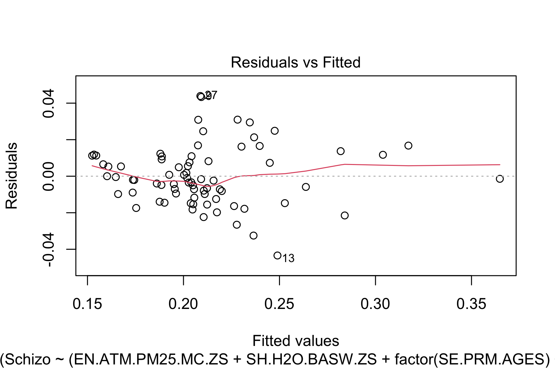Fig.3. Linear Assumption testing

R code:

ggplot(model2, aes(x=.fitted, y=.resid)) + geom_point() + geom_smooth()+ geom_hline(yintercept = 0)

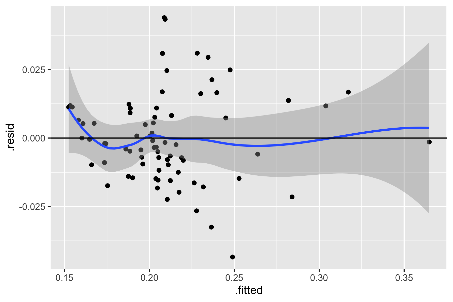Fig.4. Linear Assumption testing

Based on the plots above, we do not detect any pattern between the residuals (errors) and the fitted values (predicted). Therefore, we FAIL to reject our null hypothesis and the linearity assumption is satisfied.

Independence Assumption

$H_0$: there is no significant relationship between the independent variables $H_A$: there is a significant relationship between the independent variables

R code:

ggplot(model2, aes(x=as.numeric(row.names(model.frame(model2))), y=.resid)) + geom_point() + geom_smooth()+ geom_hline(yintercept = 0) + xlab('Number of observation') + theme(axis.text.x = element_text(angle = 90, vjust = 0.5, hjust=1))

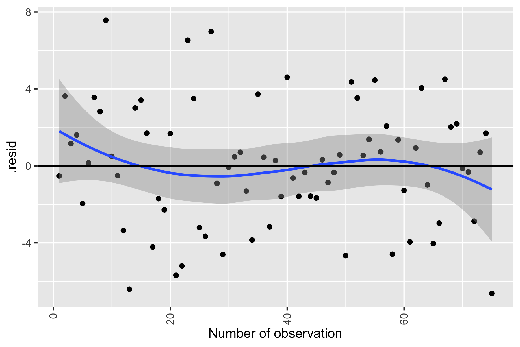Fig.5. Independence Assumption testing

There is no significant dependence of residuals on the number of observations. Thus, we FAIL to reject our null hypothesis, and the independence assumption is met for our model

Normality Assumption

$H_0$: the residuals of the model are normally distributed $H_A$: the residuals of the model are NOT normally distributed

R code:

qplot(residuals(model2), geom="histogram", binwidth = 0.01, main = "Histogram of residuals", xlab = "residuals", color="red", fill=I("blue"))

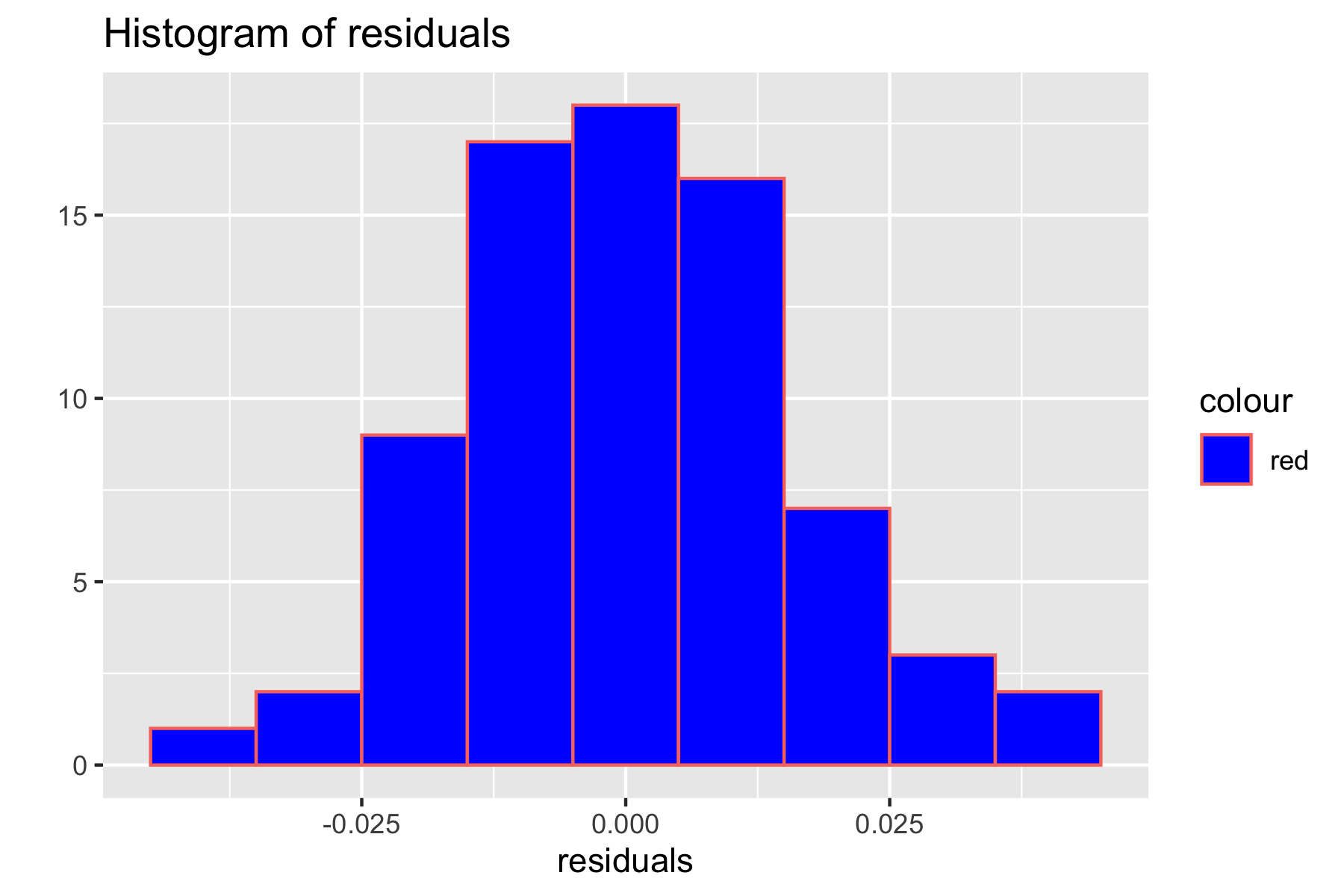Fig.6. Histogram of residuals for checking normality assumptions

R code:

ggplot(df3, aes(sample=model2$residuals)) + stat_qq() + stat_qq_line()

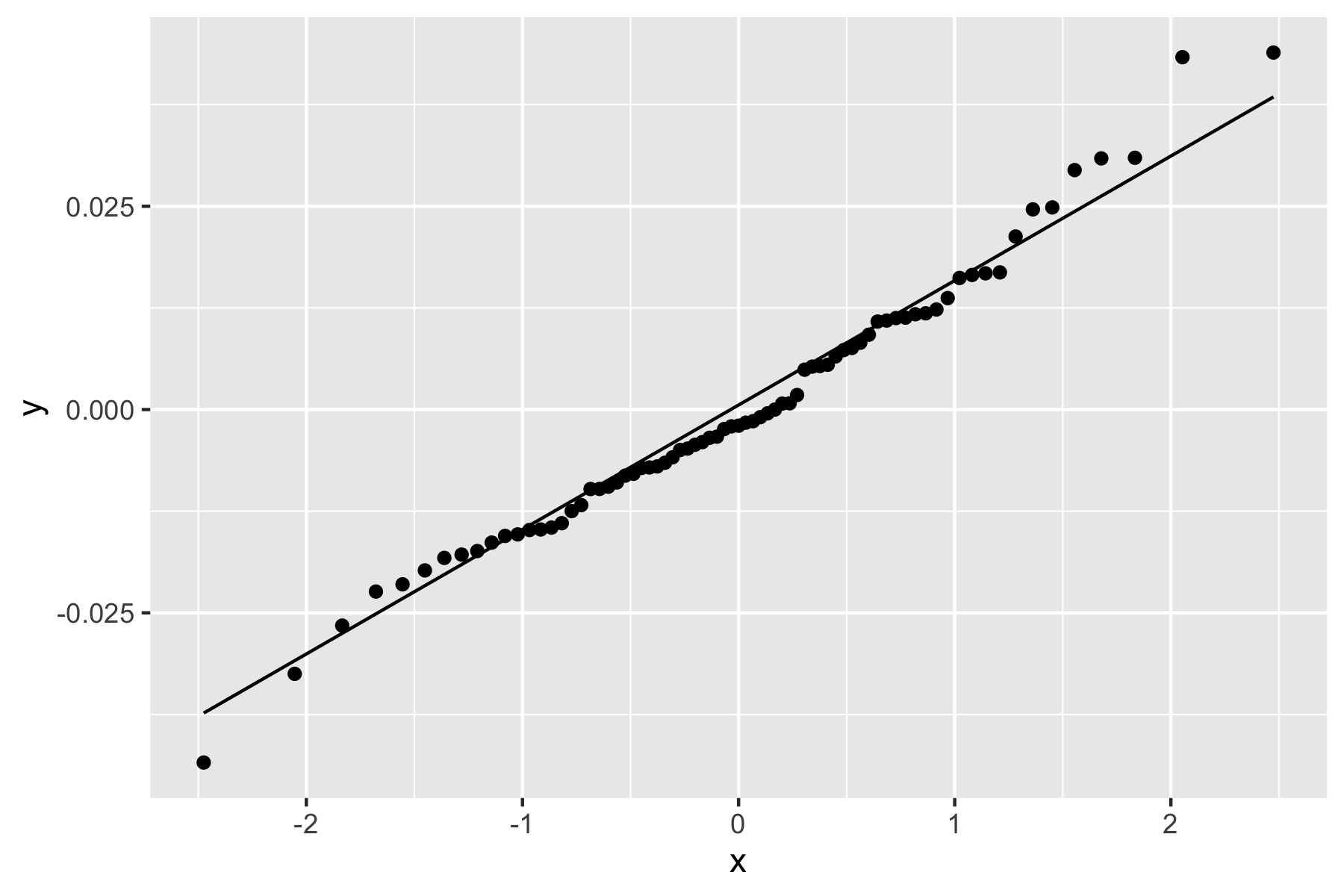QQplot Fig.7. Q-Q plot used for checking normality assumption

Based on the histogram in Figure 5, the residual distribution seems to follow a normal distribution. Additionally, the Q-Q plot also shows that the data are distributed close to the diagonal reference line. The graphs above suggest that the normality assumption is met. To further check the assumption, the Shapiro-Wilk normality test was performed:

R code:

shapiro.test(residuals(model2))

Result:

    Shapiro-Wilk normality test

data:  residuals(model2)
W = 0.98202, p-value = 0.3653

Since our p-value is greater than the significance level (0.05), we FAIL to reject our null hypothesis and conclude that the normality assumption is satisfied.

Equal Variance Assumption (homoscedasticity)

$H_0$: the residual variance is constant across the predictor variables $H_A$: the residual variance is NOT constant across the predictor variables.

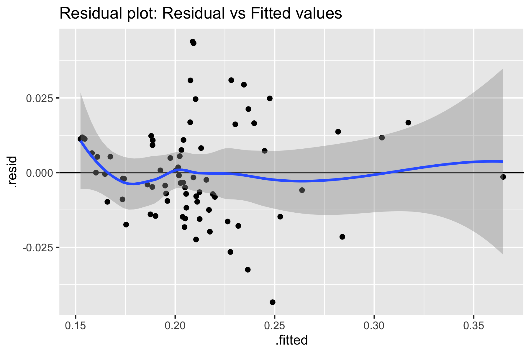Homoscedasticity Fig.8. Equal variance assumption using residual vs. fitted plot

Based on the residual plot above, we do not detect any pattern for residual distribution. Additionally, the studentized Breusch-Pagan test resulted:

R code:

bptest(model2)

Result:

    studentized Breusch-Pagan test

data:  model2
BP = 11.966, df = 8, p-value = 0.1527

Based on the residuals plot and Breusch-Pagan test we FAIL to reject our null hypothesis. Therefore, the equal variance assumption (homoscedasticity). is also satisfied.

Multicollinearity - Variance Inflation Factor

$H_0$: there is no collinearity detected in the model $H_A$: collinearity is detected in model

To test the multicollinearity we calculate Variance Inflation Factors.

R code:

imcdiag(model2, method="VIF")

Result:

Call:
imcdiag(mod = model2, method = "VIF")


 VIF Multicollinearity Diagnostics

                                  VIF detection
EN.ATM.PM25.MC.ZS              1.9957         0
SH.H2O.BASW.ZS                 1.3279         0
factor(SE.PRM.AGES)6           6.1204         0
factor(SE.PRM.AGES)7           5.8766         0
psycho_p100t                   9.7889         0
SP.URB.TOTL                    1.1043         0
beds_mhh_p100t                 1.1796         0
EN.ATM.PM25.MC.ZS:psycho_p100t 8.7863         0

NOTE:  VIF Method Failed to detect multicollinearity


0 --> COLLINEARITY is not detected by the test

Based on the VIF method in R, collinearity was NOT detected by the test. Therefore, we FAIL to reject a null hypothesis, and there is no multicollinearity in our model.

Outliers

$H_0$: there are no influential outliers in the model $H_A$: there are one or more influential outliers in the model

R code:

plot(model2, which = c(4))

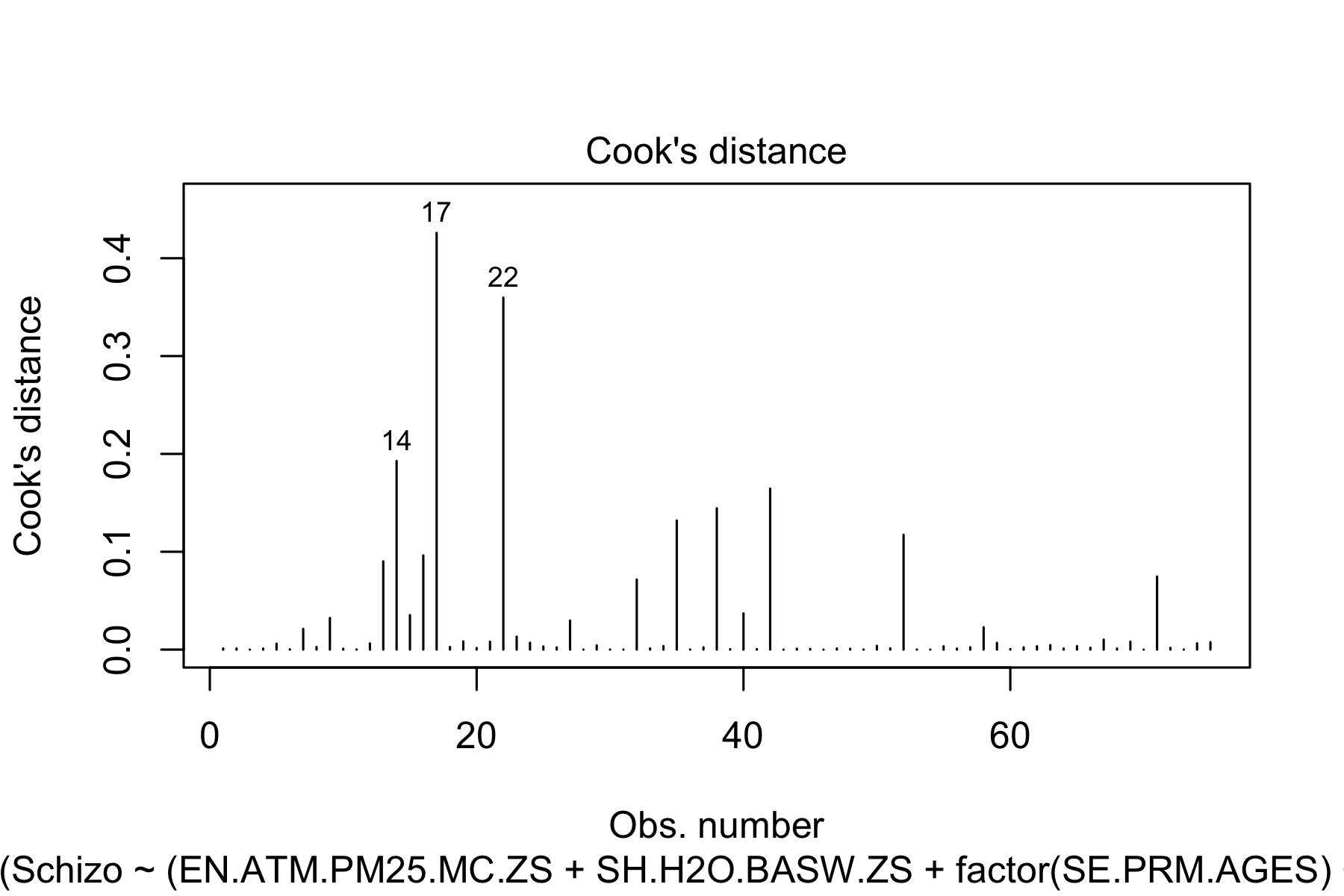Fig.9. Cook's distances

R code:

lev1=hatvalues(model2)
p = length(coef(model2))
n = nrow(df3)
plot(row.names(model.frame(model2)),lev1, main = "Leverage", xlab="observation", ylab = "Leverage Value")
abline(h = 2 *p/n, lty = 1)
abline(h = 3 *p/n, lty = 1)

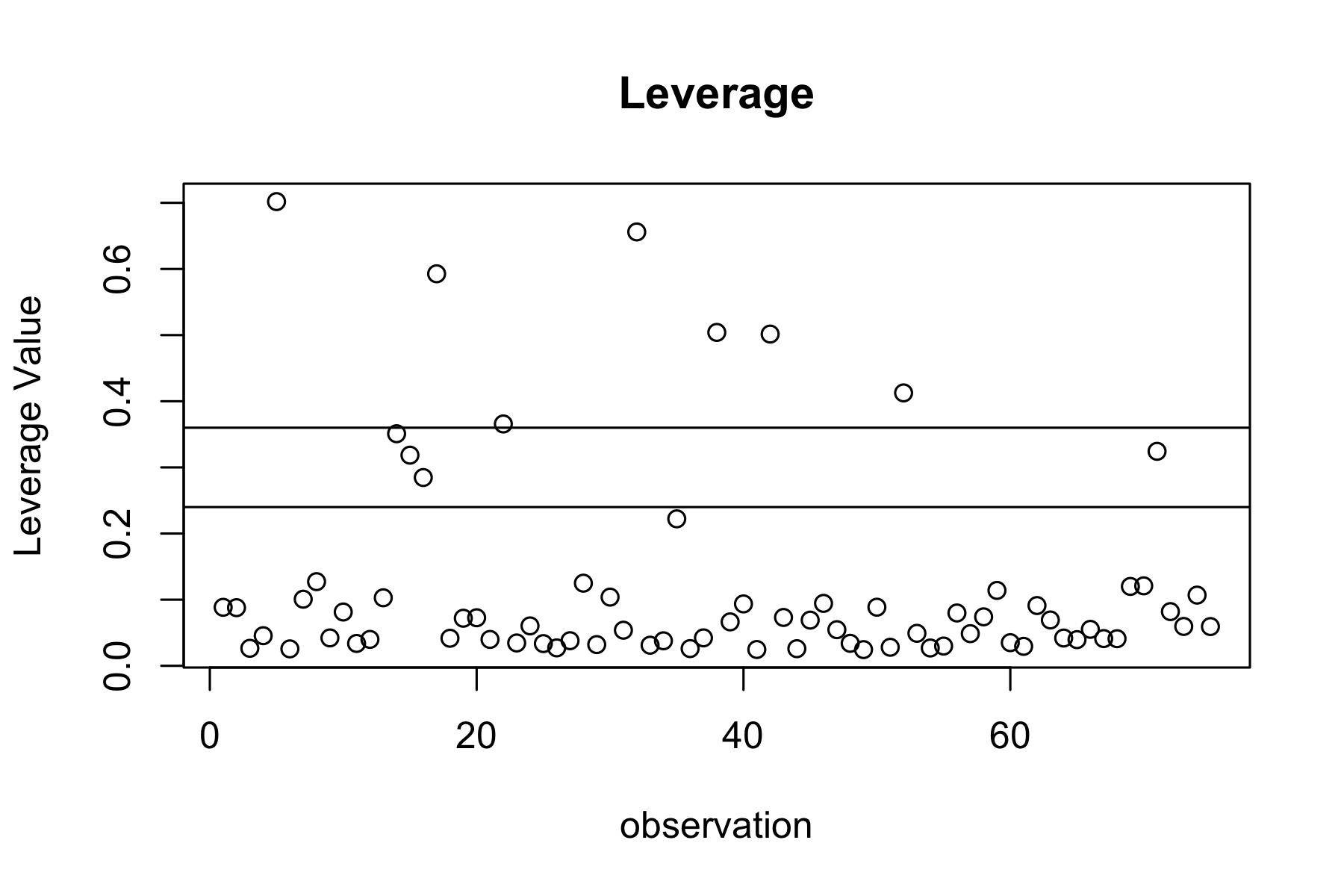Fig.10. Leverage plot

Based on the graphs above and calculations of Cook’s distances, there seem to be no influential outliers as Cook’s distance for the data points falls under Therefore, we FAIL to reject our null hypothesis and the last assumption (outliers) was also satisfied.

Conclusion

In this project, we attempted to build a model that predicts the dependence of schizophrenia prevalence on socioeconomic factors. Based on our analysis, we found the best schizophrenia model to be dependent on the following indicators

R code:

summary(model2)

Result:


Call:
lm(formula = Schizo ~ (EN.ATM.PM25.MC.ZS + SH.H2O.BASW.ZS + factor(SE.PRM.AGES) + 
    psycho_p100t + SP.URB.TOTL + beds_mhh_p100t + EN.ATM.PM25.MC.ZS:psycho_p100t), 
    data = df3)

Residuals:
      Min        1Q    Median        3Q       Max 
-0.043409 -0.009767 -0.001984  0.010884  0.043904 

Coefficients:
                                 Estimate Std. Error t value Pr(>|t|)    
(Intercept)                     1.895e-01  2.148e-02   8.822 9.01e-13 ***
EN.ATM.PM25.MC.ZS              -3.856e-04  1.126e-04  -3.424 0.001064 ** 
SH.H2O.BASW.ZS                  8.808e-04  1.531e-04   5.754 2.46e-07 ***
factor(SE.PRM.AGES)6           -3.575e-02  1.131e-02  -3.160 0.002379 ** 
factor(SE.PRM.AGES)7           -5.063e-02  1.177e-02  -4.303 5.70e-05 ***
psycho_p100t                    1.132e-03  2.441e-04   4.637 1.72e-05 ***
SP.URB.TOTL                     1.479e-10  3.284e-11   4.503 2.80e-05 ***
beds_mhh_p100t                  2.652e-04  6.801e-05   3.900 0.000228 ***
EN.ATM.PM25.MC.ZS:psycho_p100t -9.690e-06  2.815e-06  -3.443 0.001004 ** 
---
Signif. codes:  0 ‘***’ 0.001 ‘**’ 0.01 ‘*’ 0.05 ‘.’ 0.1 ‘ ’ 1

Residual standard error: 0.01722 on 66 degrees of freedom
Multiple R-squared:  0.8388,    Adjusted R-squared:  0.8193 
F-statistic: 42.94 on 8 and 66 DF,  p-value: < 2.2e-16

where:

"EN.ATM.PM25.MC.ZS : PM2.5 air pollution, population exposed to levels exceeding WHO guideline value (% of total)"
"SH.H2O.BASW.ZS : People using at least basic drinking water services (% of population)"
"SE.PRM.AGES : Primary school starting age (years)"
"psycho_p100t : Psychologists working in mental health sector (per 100,000)"
"SP.URB.TOTL : Urban population"
"beds_mhh_p100t : Beds in mental hospitals (per 100,000)"

In the future, other socioeconomic factors can be included to improve the adjusted R-squared value and the model overall. However, the model can be improved further to add other socioeconomic factors and enhance the model’s predictive power. By incorporating more variables, the model captures a broader range of factors that can contribute to Schizophrenia's prevalence, leading to a more accurate and comprehensive prediction

Gratitudes

I would like to special thank Dr. Quan Long and Dr. James McCurdy for the very useful feedback and great insights I received from the course and my project partners Shrivarshini Balaji and Niloofar Mirzadzare for productive cooperation, responsibility and excellent communication.

References

[1] Centers for Disease Control and Prevention. (2021). About mental health. Centers for Disease Control and Prevention. Retrieved from https://www.cdc.gov/mentalhealth/learn/index.htm
[2] World Health Organization. (2023). Mental health. World Health Organization. Retrieved from https://www.who.int/health-topics/mental-health#tab=tab_1
[3] World Health Organization. (2023). Schizophrenia. World Health Organization. Retrieved from https://www.who.int/news-room/fact-sheets/detail/schizophrenia
[4] American Psychiatric Association (2023). What is Schizophrenia? Retrieved from https://www.psychiatry.org/patients-families/schizophrenia/what-is-schizophrenia
[5] Johns Hopkins Medicine (2023). Schizophrenia. Retrieved from https://www.hopkinsmedicine.org/health/conditions-and-diseases/schizophrenia
[6] Brown AS. (2011). The environment and susceptibility to schizophrenia. Prog Neurobiol;93(1):23-58. doi: 10.1016/j.pneurobio.2010.09.003.
[7] World Health Organization. (2023). Global Health Estimates. World Health Organization. Retrieved from https://www.who.int/data/global-health-estimates
[8] The World Bank. (2017). World development indicators: The World Bank. World Development Indicators. Retrieved from: http://wdi.worldbank.org/table/2.12#
[9] World Health Organization. (2023). Government expenditures on mental health as a percentage of total government expenditures on Health (%). World Health Organization. Retrieved from: https://www.who.int/data/gho/data/indicators/indicator-details/GHO/government-expenditures-on-mental-health-as-a-percentage-of-total-government-expenditures-on-health-(-)